\(\DeclareMathOperator{\Div}{div}
\DeclareMathOperator{\Rot}{rot}
\newcommand{\parder}[2]{\frac{\partial {#1}}{\partial {#2}}}\)$\setCounter{0}$

This post should be a straightforward walkthrough of the Berreman’s paper¹ using the approach we implemented in the previous posts, that is: minimizing the amount of constants by working in the HL system of units and using the geometrical components of the wave-vectors. It should be stated that the original paper is already very clear in this respect. In this post we will follow it up to the point where \(\mathbf{\hat{S}}\) matrix and \(\boldsymbol{\hat{\Delta}}\) matrix are defined – and remove one unnecessary minus.

In following blog post we will treat the interface and discuss some practical questions of wave propagation in quadrochromic thin films and multilayers.

Maxwell equations in 6×6 form

We start from scratch with Maxwell’s equations in the form as seen before:

\(\begin{align}
\begin{aligned}
\Div\mathbf{D} &=0, &\Div\mathbf{B} &=0,
\\
-\Rot\mathbf{E} &=\frac{1}{c}\parder{\mathbf{B}}{t}, &\Rot\mathbf{H} &=\frac{1}{c}\parder{\mathbf{D}}{t} .
\end{aligned}
\end{align}\)

So only the curly part of the electro-magnetic field is of interest, and the corresponding two equations can be written explicitly in a 6×6 matrix form:

\(
\begin{align}
\begin{bmatrix}
0 & 0 & 0 & 0 & -\parder{}{z} & \parder{}{y} \\
0 & 0 & 0 & \parder{}{z} & 0 & -\parder{}{x} \\
0 & 0 & 0 & -\parder{}{y} & \parder{}{x} & 0 \\
0 & \parder{}{z} & -\parder{}{y} & 0 & 0 & 0 \\
-\parder{}{z} & 0 & \parder{}{x} & 0 & 0 & 0 \\
\parder{}{y} & -\parder{}{x} & 0 & 0 & 0 & 0
\end{bmatrix}
\begin{bmatrix}
E_x \\ E_y \\ E_z \\ H_x \\ H_y \\ H_z
\end{bmatrix}
=
\frac{1}{c}\parder{}{t}
\begin{bmatrix}
D_x \\ D_y \\ D_z \\ B_x \\ B_y \\ B_z
\end{bmatrix}.
\end{align}
\)

We will use the same abbreviation as Berreman:

\(\begin{align}\label{eqRGC}
\mathbf{\hat{R}}\mathbf{G}=\frac{1}{c}\parder{}{t}\mathbf{C},
\end{align}\)

where \(\mathbf{\hat{R}}\) is the rotation differential operator, \(\bf{G}\) is the vector of electric and magnetic fields and \(\bf{C}\) is the vector of the electric displacement and magnetic induction. The constitutive relations will have a general form:

\(\begin{align}
\begin{aligned}
\mathbf{D} &=\boldsymbol{\hat{\varepsilon}}\mathbf{E} + \boldsymbol{\hat{\rho}}\mathbf{H},
\\
\mathbf{B} &=\boldsymbol{\hat{\mu}}\mathbf{H}+ \boldsymbol{\hat{\rho}’}\mathbf{E}.
\end{aligned}
\end{align}\)

explicitly as

\(
\begin{align}
\begin{bmatrix}
D_x \\ D_y \\ D_z \\ B_x \\ B_y \\ B_z
\end{bmatrix}
=
\begin{bmatrix}
\varepsilon_{11} & \varepsilon_{12} & \varepsilon_{13} & \rho_{11} & \rho_{12} & \rho_{13} \\
\varepsilon_{21} & \varepsilon_{22} & \varepsilon_{23} & \rho_{21} & \rho_{22} & \rho_{23} \\
\varepsilon_{31} & \varepsilon_{32} & \varepsilon_{33} & \rho_{31} & \rho_{32} & \rho_{33} \\
\rho_{11}’ & \rho_{12}’ & \rho_{13}’ & \mu_{11} & \mu_{12} & \mu_{13} \\
\rho_{21}’ & \rho_{22}’ & \rho_{23}’ & \mu_{21} & \mu_{22} & \mu_{23} \\
\rho_{31}’ & \rho_{32}’ & \rho_{33}’ & \mu_{31} & \mu_{32} & \mu_{33}
\end{bmatrix}
\begin{bmatrix}
E_x \\ E_y \\ E_z \\ H_x \\ H_y \\ H_z
\end{bmatrix},
\end{align}
\)

abbreviated as

\(\begin{align}\label{eqCMG}
\mathbf{C}=\mathbf{\hat{M}}\mathbf{G},
\end{align}\)

with \(\mathbf{\hat{M}}\) being the material’s linear response tensor, written in a coordinate system defined below.

Stationary solution

We will immediatelly assume homogeneous bulk and search for a solution of \eqref{eqRGC} with \eqref{eqCMG} in the form of plane waves

\(\begin{align}\label{eqKaGamma}
\mathbf{G}=\boldsymbol{\Gamma} e^{i(\mathbf{kr}-\omega t)} ,
\end{align}\)

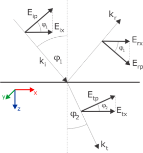
where \(\boldsymbol{\Gamma}\) is the vector of field amplitudes and we will want to choose the coordinate system so the wave \(\mathbf{k}\) propagates in the x-z plane as we are used to. We also introduce the geometrical components:

\(\begin{align}\label{eqKaxiq}
\mathbf{k}=\frac{\omega}{c}\boldsymbol{\kappa} = \frac{\omega}{c}(\xi,0,q),
\end{align}\)

where \(\xi\) is the conserved real x-component of the wave-vector and we will need to find possible \(q\), the z-components, just like we did in the Part 2 of the isotropic problem, only here we will keep Berreman’s notation \(q\) for the z-components. There will be 4 solutions and for each of them we will find the corresponding amplitude/polarization vector.

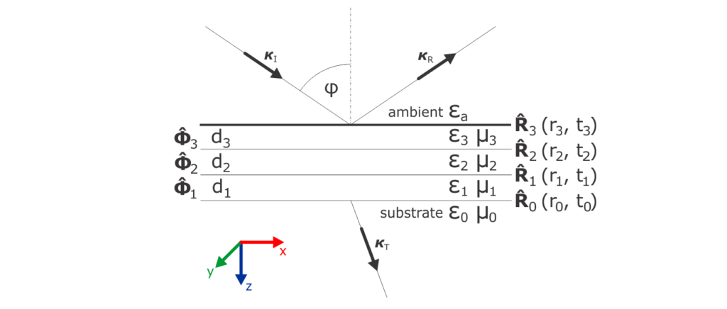
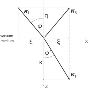
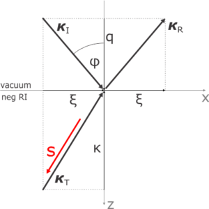
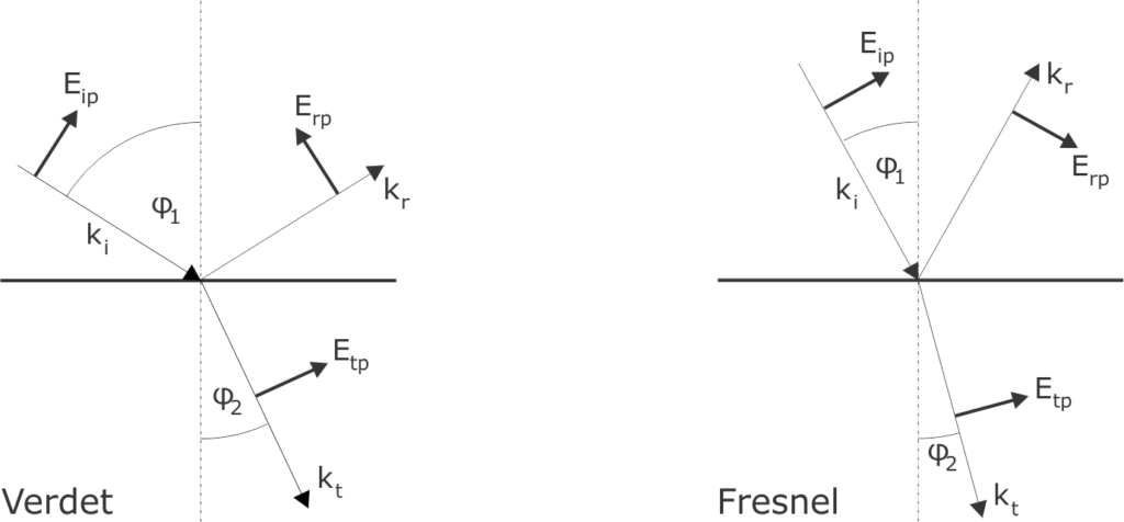
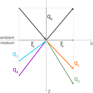
The following figure illustrates the situation. Althought, at this point, we simply look for the modes possible in the bulk, we will later couple them through interfaces to the ambient. In the transparent ambient we are able to set and measure the real angle of incidence, which fixes the invariant \(\xi\). The angle of refraction loses clear sense in an absorbing medium, as it would need to be expressed as complex quantity. That is due to the fact that the wave vector becomes complex, but its imaginary parts have only z-component – as the x-component \(\xi\) is real and conserved. Moreover, the angle of refraction is hardly ever needed for understanding the ellipsometeric experiment.

The problem we will be solving is an eigen-problem, and the four possible z-components of the wave-vector are eigenvalues of some operator – to which we will arrive at the end of this post. The eigenvectors associated with the eigenvalues describe the polarization states that propagate through the medium without change, apart from evolving phase and decreasing amplitude. For example, linearly polarized light in solution of some sugars will experience rotation of the polarization direction – so it is not the polarization eigen-state of such medium. But there will be a circular polarization that propagates and stays circular, experiencing certain refractive index, while the opposite circular polarization also stays in its state, just experiencing different refractive index. That is called the circular birefringence.

The Berreman’s method is an expansion of the simple isotropic case, where we found that for both linear polarizations, the z-component of the wave-vector was \(q=\pm\sqrt{\varepsilon\mu-\xi^2}\), with the right sign for the down- and up-propagating mode. The material response tensor \(\mathbf{\hat{M}}\) has some physical constrains, but can lead to situations where the four modes (two down and two up) propagating in the medium have distinct properties and carry generally elliptical polarization states. Such general media are called quadrochromic in the litarature.

On the left-hand side of equation \eqref{eqRGC} we apply the differential operator \(\mathbf{\hat{R}}\) on the vector \(\mathbf{G}\) in the form of equation \eqref{eqKaGamma}, with the wave-vector \eqref{eqKaxiq}, obtaining:

\(
\begin{align}
\mathbf{\hat{R}}\mathbf{G}=
i\frac{\omega}{c}
\begin{bmatrix}
0 & 0 & 0 & 0 & -q & 0 \\
0 & 0 & 0 & q & 0 & -\xi \\
0 & 0 & 0 & 0 & \xi & 0 \\
0 & q & 0 & 0 & 0 & 0 \\
-q & 0 & \xi & 0 & 0 & 0 \\
0 & -\xi & 0 & 0 & 0 & 0
\end{bmatrix}
\boldsymbol{\Gamma} e^{i(\mathbf{kr}-\omega t)}.
\end{align}
\)

On the right-hand side of \eqref{eqRGC} we apply the time derivative on the displacement-induction vector \(\mathbf{C}\), while the response tensor \(\mathbf{\hat{M}}\) is constant.

\(\begin{align}
\frac{1}{c}\parder{}{t}\mathbf{C} = \frac{1}{c}\mathbf{\hat{M}}\parder{}{t}\mathbf{G} = -i\frac{\omega}{c}\mathbf{\hat{M}}\boldsymbol{\Gamma} e^{i(\mathbf{kr}-\omega t)}.
\end{align}\)

Now we combine the last two expressions, cancel the constants and the non-zero complex exponential factor. In that we have converted the differential physical problem to a dimensionless, algebraic or geometrical, one.

\(
\begin{align}\label{eqGMG}
\begin{bmatrix}
0 & 0 & 0 & 0 & -q & 0 \\
0 & 0 & 0 & q & 0 & -\xi \\
0 & 0 & 0 & 0 & \xi & 0 \\
0 & q & 0 & 0 & 0 & 0 \\
-q & 0 & \xi & 0 & 0 & 0 \\
0 & -\xi & 0 & 0 & 0 & 0
\end{bmatrix}
\boldsymbol{\Gamma}
=
-\mathbf{\hat{M}}\boldsymbol{\Gamma}.
\end{align}
\)

In this equation, the unknowns are \(q\) – the geometric z-component of the wave-vector – and the elements of \(\boldsymbol{\Gamma}\), the electric and magnetic field amplitudes, which both have the same unit in HLU. It is immediatelly apparent that the fields vector will be found up to a constant prefactor. It describes a polarization state, so multiplying it by constant does not change the state. What follows now is simply commented algebra.

Reduction to 4×4 form

First we extract the 3^rd and 6^th rows as they do not contain \(q\), and have on the right hand side the \(D_z\) and \(B_z\) components. As before, we will be interested in the state of the in-plane, xy-components of the fields, even we did not yet defined any interface. Taking apart the two rows allows us to separate the \(E_z\) and \(H_z\) components.

So the third and sixth rows yield:

\(\begin{align}
\begin{aligned}
\xi\Gamma_5 &= -\sum_{j=1}^{6} M_{3j}\Gamma_j,
\\
\xi\Gamma_2 &= \sum_{j=1}^{6} M_{6j}\Gamma_j.
\end{aligned}
\end{align}\)

We write this explicitly, separate the \(\Gamma_3\) and \(\Gamma_6\) and define shorthand symbols \(A_3\) and \(A_6\).

\(\begin{align}
\begin{aligned}
\overbrace{ -M_{31}\Gamma_1 – M_{32}\Gamma_2 – M_{34}\Gamma_4 – (M_{35}+ \xi)\Gamma_5 }^{A_3} &= M_{33}\Gamma_3 + M_{36}\Gamma_6 ,
\\
\overbrace{ -M_{61}\Gamma_1 – (M_{62}- \xi)\Gamma_2 – M_{64}\Gamma_4 – M_{65}\Gamma_5 }^{A_6} &= M_{63}\Gamma_3 + M_{66}\Gamma_6 .
\end{aligned}
\end{align}\)

Then

\(\begin{align}\label{eqDMM}
D \equiv M_{33}M_{66} – M_{36}M_{63},
\end{align}\)

and the solution for \(\Gamma_3 \equiv E_z\) and \(\Gamma_6 \equiv H_z\) is

\(\begin{align}
\Gamma_3 = \frac{M_{66}A_{3} – M_{36}A_{6}}{D} , \quad \Gamma_6 = \frac{M_{33}A_{6} – M_{63}A_{3}}{D}.
\end{align}\)

We will rewrite the solutions with new shorthand symbols \(a_{mn}\) as:

\(\begin{align}
\begin{aligned}
\Gamma_3 &= a_{31}\Gamma_{1} + a_{32}\Gamma_{2} + a_{34}\Gamma_{4} + a_{35}\Gamma_{5} ,
\\
\Gamma_6 &= a_{61}\Gamma_{1} + a_{62}\Gamma_{2} + a_{64}\Gamma_{4} + a_{65}\Gamma_{5} ,
\end{aligned}
\label{eqG3G6}
\end{align}\)

where the \(a_{mn}\) are just various combinations of the material response tensor elements, some modified by \(\xi\).

\(\begin{align}
\begin{aligned}
a_{31} &= \frac{1}{D} ( -M_{31}M_{66} + M_{61}M_{36} ), \\
a_{32} &= \frac{1}{D} ( -M_{32}M_{66} + (M_{62}-\xi)M_{36} ), \\
a_{34} &= \frac{1}{D} ( -M_{34}M_{66} + M_{64}M_{36} ), \\
a_{35} &= \frac{1}{D} ( -(M_{35}+\xi)M_{66} + M_{65}M_{36} ), \\
a_{61} &= \frac{1}{D} ( -M_{61}M_{33} + M_{31}M_{63} ), \\
a_{62} &= \frac{1}{D} ( -(M_{62}-\xi)M_{33} + M_{32}M_{63} ), \\
a_{64} &= \frac{1}{D} ( -M_{64}M_{33} + M_{34}M_{63} ), \\
a_{65} &= \frac{1}{D} ( -M_{65}M_{33} + (M_{35}+\xi)M_{63} ).
\end{aligned}
\end{align}\)

Note that some important role is played by the \(D\), defined above in \eqref{eqDMM} as a combination of the zz-elements of the tensors \(\boldsymbol{\hat{\varepsilon}}\), \(\boldsymbol{\hat{\mu}}\), \(\boldsymbol{\hat{\rho}}\) and \(\boldsymbol{\hat{\rho}’}\). We will have to assume that \(D\neq 0\), which – in most common cases – means non-zero \(\varepsilon_{33}\). Curious effects can develop when the \(\varepsilon_{33}\), or \(D\), are near-zero. Those are called Berreman’s effects, but in reference to another Berreman’s cornerstone paper.² We shall discuss them separately later.

Now we can write the remaining four equations from eq. \eqref{eqGMG} as

\(
\begin{align}
q
\begin{bmatrix}
0 & 0 & 0 & -1 \\
0 & 0 & 1 & 0 \\
0 & 1 & 0 & 0 \\
-1 & 0 & 0 & 0
\end{bmatrix}
\begin{bmatrix}
\Gamma_1 \\ \Gamma_2 \\ \Gamma_4 \\ \Gamma_5
\end{bmatrix}
=-
\begin{bmatrix}
\sum M_{1j}\Gamma_j \\
\sum M_{2j}\Gamma_j – \xi\Gamma_6 \\
\sum M_{4j}\Gamma_j \\
\sum M_{5j}\Gamma_j – \xi\Gamma_3
\end{bmatrix}
\equiv
-\mathbf{\hat{S}}
\begin{bmatrix}
\Gamma_1 \\ \Gamma_2 \\ \Gamma_4 \\ \Gamma_5
\end{bmatrix},
\label{eqqSGamma}
\end{align}\)

where we inserted the \(\Gamma_3\) and \(\Gamma_6\) from \eqref{eqG3G6} and defined the \(\mathbf{\hat{S}}\) matrix identical to Berreman’s manuscript:

\( \small{
\mathbf{\hat{S}}
=
\begin{bmatrix}
M_{11} + M_{13}a_{31} + M_{16}a_{61} & M_{12} + M_{13}a_{32} + M_{16}a_{62} & M_{14} + M_{13}a_{34} + M_{16}a_{64} & M_{15} + M_{13}a_{35} + M_{16}a_{65} \\
M_{21} + M_{23}a_{31} + (M_{26}-\xi)a_{61} & M_{22} + M_{23}a_{32} + (M_{26}-\xi)a_{62} & M_{24} + M_{23}a_{34} + (M_{26}-\xi)a_{64} & M_{25} + M_{23}a_{35} + (M_{26}-\xi)a_{65} \\
M_{41} + M_{43}a_{31} + M_{46}a_{61} & M_{42} + M_{43}a_{32} + M_{46}a_{62} & M_{44} + M_{43}a_{34} + M_{46}a_{64} & M_{45} + M_{43}a_{35} + M_{46}a_{65} \\
M_{51} + (M_{53}+\xi)a_{31} + M_{56}a_{61} & M_{52} + (M_{53}+\xi)a_{32} + M_{56}a_{62} & M_{54} + (M_{53}+\xi)a_{34} + M_{56}a_{64} & M_{55} + (M_{53}+\xi)a_{35} + M_{56}a_{65}
\end{bmatrix}.
} \)

Reorganize to get Delta form

Now we just reorganize the rows and colums, and extinguish minuses. In the field components, the equation \eqref{eqqSGamma} reads

\(
\begin{align}
q
\begin{bmatrix}
-H_y \\ H_x \\ E_y \\ -E_x
\end{bmatrix}
=
-\mathbf{\hat{S}}
\begin{bmatrix}
E_x \\ E_y \\ H_x \\ H_y
\end{bmatrix}.
\end{align}\)

We will interchange the first, second and last row of the whole system, then swap second, third and last column of the matrix on the right hand side. Finally, we switch some minuses obtaining

\(
\begin{align}
q
\begin{bmatrix}
E_x \\ H_y \\ E_y \\ H_x
\end{bmatrix}
=
\overbrace{
\begin{bmatrix}
S_{41} & S_{44} & S_{42} & S_{43} \\
S_{11} & S_{14} & S_{12} & S_{13} \\
-S_{31} & -S_{34} & -S_{32} & -S_{33} \\
-S_{21} & -S_{24} & -S_{22} & -S_{23}
\end{bmatrix}}^{\boldsymbol{\hat{\Delta}}}
\overbrace{
\begin{bmatrix}
E_x \\ H_y \\ E_y \\ H_x
\end{bmatrix}}^{\boldsymbol{\Psi}},
\end{align}\)

which defines the \(\boldsymbol{\hat{\Delta}}\) matrix and fixes the order of polarization state vector \(\boldsymbol{\Psi}\). Note that the order of the components of \(\boldsymbol{\Psi}\) is rather arbitrary, and is chosen so the components of linear p- and s- polarizations appear together in sub-blocks.

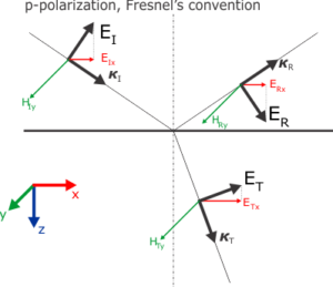
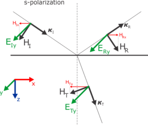
Berreman introduced additional minus in front of the \(H_x\) component, which is related to s-polarization and served merely esthetical purposes: In the right-handed media and wave propagating along z-axis, the p-polarization with positive \(E_x\) amplitude will have positive \(H_y\), but s-polarization with positive \(E_y\) will have negative \(H_x\). Placing the minus there will therefore obliterate some minuses when later solving simple problems in semi-infinite media. Schubert³ defined the \(\boldsymbol{\Psi}\) vector without the decorative minus, but in different order of components.

We have now our eigenproblem:

\(\begin{align} q\boldsymbol{\Psi} = \boldsymbol{\hat{\Delta}}\boldsymbol{\Psi}, \end{align}\)

with \(\boldsymbol{\hat{\Delta}}\) matrix explicitly:

\( \small{
\boldsymbol{\hat{\Delta}}
=
\begin{bmatrix}
M_{51} +(M_{53}+\xi)a_{31} +M_{56}a_{61} & M_{55} +(M_{53}+\xi)a_{35} +M_{56}a_{65} & M_{52} +(M_{53}+\xi)a_{32} +M_{56}a_{62} & M_{54} +(M_{53}+\xi)a_{34} +M_{56}a_{64} \\
M_{11} +M_{13}a_{31} +M_{16}a_{61} & M_{15} +M_{13}a_{35} +M_{16}a_{65} & M_{12} +M_{13}a_{32} +M_{16}a_{62} & M_{14} +M_{13}a_{34} +M_{16}a_{64} \\
-M_{41} -M_{43}a_{31} -M_{46}a_{61} & -M_{45} -M_{43}a_{35} -M_{46}a_{65} & -M_{42} -M_{43}a_{32} -M_{46}a_{62} & -M_{44} -M_{43}a_{34} -M_{46}a_{64} \\
-M_{21} -M_{23}a_{31} -(M_{26}-\xi)a_{61} & -M_{25} -M_{23}a_{35} -(M_{26}-\xi)a_{65} & -M_{22} -M_{23}a_{32} -(M_{26}-\xi)a_{62} & -M_{24} -M_{23}a_{34} -(M_{26}-\xi)a_{64}
\end{bmatrix}.
} \)

Inserting the response tensor

And since internet is realy huge, we can occupy some more space by expressing everything in the original response tensors:

\(\begin{align}
D = \varepsilon_{33}\mu_{33} – \rho_{33}\rho_{33}’,
\end{align}\)

\(\begin{align}
\begin{aligned}
a_{31} &= \frac{1}{D} ( -\varepsilon_{31}\mu_{33} + \rho_{31}’\rho_{33} ), \\
a_{32} &= \frac{1}{D} ( -\varepsilon_{32}\mu_{33} + (\rho_{32}’-\xi)\rho_{33} ), \\
a_{34} &= \frac{1}{D} ( -\rho_{31}\mu_{33} + \mu_{31}\rho_{33} ), \\
a_{35} &= \frac{1}{D} ( -(\rho_{32}+\xi)\mu_{33} + \mu_{32}\rho_{33} ), \\
a_{61} &= \frac{1}{D} ( -\rho_{31}’\varepsilon_{33} + \varepsilon_{31}\rho_{33}’ ), \\
a_{62} &= \frac{1}{D} ( -(\rho_{32}’-\xi)\varepsilon_{33} + \varepsilon_{32}\rho_{33}’ ), \\
a_{64} &= \frac{1}{D} ( -\mu_{31}\varepsilon_{33} + \rho_{31}\rho_{33}’ ), \\
a_{65} &= \frac{1}{D} ( -\mu_{32}\varepsilon_{33} + (\rho_{32}+\xi)\rho_{33}’ ).
\end{aligned}
\end{align}\)

\( \small{
\boldsymbol{\hat{\Delta}}
=
\begin{bmatrix}
\rho_{21}’ +(\rho_{23}’+\xi)a_{31} +\mu_{23}a_{61} & \mu_{22} +(\rho_{23}’+\xi)a_{35} +\mu_{23}a_{65} & \rho_{22}’ +(\rho_{23}’+\xi)a_{32} +\mu_{23}a_{62} & \mu_{21} +(\rho_{23}’+\xi)a_{34} +\mu_{23}a_{64} \\
\varepsilon_{11} +\varepsilon_{13}a_{31} +\rho_{13}a_{61} & \rho_{12} +\varepsilon_{13}a_{35} +\rho_{13}a_{65} & \varepsilon_{12} +\varepsilon_{13}a_{32} +\rho_{13}a_{62} & \rho_{11} +\varepsilon_{13}a_{34} +\rho_{13}a_{64} \\
-\rho_{11}’ -\rho_{13}’a_{31} -\mu_{13}a_{61} & -\mu_{12} -\rho_{13}’a_{35} -\mu_{13}a_{65} & -\rho_{12}’ -\rho_{13}’a_{32} -\mu_{13}a_{62} & -\mu_{11} -\rho_{13}’a_{34} -\mu_{13}a_{64} \\
-\varepsilon_{21} -\varepsilon_{23}a_{31} -(\rho_{23}-\xi)a_{61} & -\rho_{22} -\varepsilon_{23}a_{35} -(\rho_{23}-\xi)a_{65} & -\varepsilon_{22} -\varepsilon_{23}a_{32} -(\rho_{23}-\xi)a_{62} & -\rho_{21} -\varepsilon_{23}a_{34} -(\rho_{23}-\xi)a_{64}
\end{bmatrix}.
} \)

In some future post, we will continue with stratified media and coupling to the ambient through the interface.

---

¹ D. W. Berreman, Optics in Stratified and Anistropic Media: 4×4-Matrix Formulation, Journal of the Optical Society of America, vol 62, 4 (1972).
² D. W. Berreman, Infrared Absorption at Longitudinal Optic Frequency in Cubic Crystal Films, Physical Review, vol 130, 6 (1963).
³ M. Schubert, Polarization-dependent optical parameters of arbitrarily anisotropic homogeneous layered systems, Physical Review B, vol 53, 8 (1996).

$\setCounter{0}$
Part 1: The wave vector
Part 2: The interface
Part 3: The s-polarization
Part 4: The p-polarization
Part 5: Multilayers

Although we have already finished with what was promised at the beginning of this series – that is, we have derived the Fresnel’s coefficients for isotropic semi-infinite \(\varepsilon\mu\) medium in vacuum – we can now, with little effort, generalize the findings for a multi-layered system on semi-infinite substrate and surrounded by transparent dielectric medium. We will assume that the ambient medium is simple transparent dielectric with real \(\varepsilon_{a} > 0\), and our films and substrate consist of isotropic \(\varepsilon\mu\) materials.

Multilayer stack

The following sketch presents such multilayer with three films on substrate, but our formalism can be easily extended for any finite number of layers.

We will be indexing our layers with \(j=0..3\), so the substrate response functions will be denoted as \(\varepsilon_0\), \(\mu_0\), not to be confused with vacuum permittivity and permeability constants.¹ The ambient properties should have, technically, index \(j=4\) here, i.e \(\varepsilon_4 \equiv \varepsilon_{a}\), and \(\mu_4 \equiv \mu_{a} = 1\). The index \(j\) also belongs to thickness \(d_j\) of the particular layer and identifies the interface on top of that layer. The meaning of the symbols \(\mathbf{\hat{R}}_j\), \(\boldsymbol{\hat{\Phi}}_j\) will become clear below. We also illustrated the incident, \(\boldsymbol{\kappa}_I\), and reflected, \(\boldsymbol{\kappa}_R\), waves, together with the final transmitted wave, \(\boldsymbol{\kappa}_T\), which travels into the semi-infinite substrate.

Wave vectors in layers

In the transparent ambient, we can well define the angle of incidence \(\varphi\) and calculate the constants \(q = n_{a}\cos{\varphi}\) and \(\xi = n_{a}\sin{\varphi}\), where \(n_{a} = \sqrt{\varepsilon_{a}}\) is the ambient refractive index. Most typical scenario is, of course, vacuum or air ambient with \(n_a = 1\), but apart from that, we could be having some glass prism or immersion liquid medium with \(n_a > 1\) on top of our sample. Important point here is that \(\xi\), the x-component of the wave vector is conserved across all interfaces, i.e. remains real and non-negative. Then we can immediately calculate \(\kappa_j\), the z-component for any layer, inc. the substrate:

\( \begin{align}\label{eqKappaj} \kappa_j = \sqrt{\varepsilon_j \mu_j – \xi^2}, \end{align} \)

which is valid also for the ambient, where \(\kappa_4 \equiv q\). Now we should consider again which root should be taken. In fact, for all the films and given \(\xi\), there are two possible wave vectors, one with \(\kappa_j\) and one with \(-\kappa_j\). The letter belongs to a wave reflected from lower interface and propagating upwards. We will choose the down-propagating wave vector component \(\kappa_j\) based on the imaginary part of the square-root, which must be positive. In case both \(\varepsilon_j\) and \(\mu_j\) are real, negative, and the argument of the square-root remains positive, we have to choose the negative real root as \(\kappa_j\), since we have negative refraction.

General Fresnel’s coefficients

Now we will write the Fresnel’s coefficients for any interface between medium A and medium B, as schematically sketched below.

Note that A is the upper medium and B the lower, so when compared to the first figure in this post, we should not confuse the indexing. For example, the topmost interface will have \(A=4\) and \(B=3\), etc.

\( \begin{align} \begin{aligned} &\text{p-polarized}\quad &r_{xAB} &= \frac{\varepsilon_A \kappa_B – \varepsilon_B \kappa_A}{\varepsilon_A \kappa_B + \varepsilon_B \kappa_A}, &t_{xAB} &= \frac{2 \varepsilon_A \kappa_B}{\varepsilon_A \kappa_B + \varepsilon_B \kappa_A}, \\ \\ &\text{s-polarized}\quad &r_{yAB} &= \frac{\mu_B \kappa_A – \mu_A \kappa_B}{\mu_B \kappa_A + \mu_A \kappa_B}, &t_{yAB} &= \frac{2 \mu_B \kappa_A}{\mu_B \kappa_A + \mu_A \kappa_B}, \end{aligned}\label{eqsFresnelsGeneral} \end{align} \)

where we labeled the coefficients with \(x\) and \(y\) to highlight that we are using our definitions in terms of the in-plane, \(x\) and \(y\), components of the electric field.

We should notice that \(r_{AB} = -r_{BA}\), i.e. that Fresnel’s reflection coefficient from the other side of the interface is exactly opposite, and that is true for both polarizations. Let’s simplify our notation again, and mark the reflection coefficient from above as \(r\), the reflection from below as \(r’\), the transmission from top as \(t\), and transmission from below upwards as \(t’\).

So we have \( r’ = -r \), and also \(1+r=t\), as well as \(1+r’ = t’\), valid for both polarizations, which can be put together to obtain \(1-r^2 = tt’\). This identity we will use in a moment.

Interface matrix

When we look at any of the interfaces, we will see that now we have to match four waves, \(\boldsymbol{\kappa}_I\), \(\boldsymbol{\kappa}_R\), \(\boldsymbol{\kappa}_T\) and \(\boldsymbol{\kappa}_B\) (\(B\) as back-propagating wave). The wave vectors all share the same x-component \(\xi\), since they all originate from the same topmost incident wave. The \(\boldsymbol{\kappa}_B\) is just reflected from some interfaces below. So in each layer, the electromagnetic field is composed of two waves for single polarization (we treat the polarizations separately here), one propagating down with the pre-calculated z-component \(\kappa_j \) (eq. \eqref{eqKappaj}) and other propagating up with \(-\kappa_j \).

Remember that the basic optics textbook explanation of thin film interference would discuss multiple reflections, which form infinite geometric series that gets eventually summed into single term. What we are developing here is the standard transfer matrix formalism, which is completely compatible, but we start from the idea that we have already only the pair of down and up propagating modes in any layer, and look for the linear coupling coefficients to match the waves on the interfaces.

On each interface, the tangential, x- or y-components of the electric field amplitudes must satisfy the continuity condition. In the following, we drop the corresponding index \(x\) or \(y\), since the formulas are valid for both polarizations:

\(
\begin{align}
E_I + E_R = E_T + E_B.
\end{align}
\)

We will reuse the already derived Fresnel’s coefficients, and write the amplitude \(E_R\) of the reflected wave as composed form the reflected part of the incident wave \(E_I\) and part of the \(E_B\) wave transmitted from below:

\(
\begin{align}\label{eqErEiEb}
E_R = rE_I + t’E_B.
\end{align}
\)

Also the total \(E_T\) is sum of the transmitted part of the incident wave \(E_T\) and back-reflected part of \(E_B\):

\(
\begin{align}\label{eqEtEiEb}
E_T = tE_I + r’E_B.
\end{align}
\)

We will want to express the fields above the interface, \(E_I\), \(E_R\) as combination of the waves below, \(E_T\), \(E_B\). So from \eqref{eqEtEiEb}, using \(r’ = -r\),

\(
\begin{align}\label{eqEiEtEb}
E_I = \frac{1}{t} (E_T – r’E_B) = \frac{1}{t} (E_T + rE_B),
\end{align}
\)

which we directly plug to \eqref{eqErEiEb}

\(
\begin{align}\label{eqErEtEb}
E_R =\frac{r}{t}(E_T + rE_B) + t’E_B = \frac{1}{t} (rE_T + r^2E_B + tt’E_B) = \frac{1}{t} (rE_T + E_B ),
\end{align}
\)

where we used the identity \(r^2 + tt’ = 1\) presented above. We will want to write eqs. \eqref{eqEiEtEb} and \eqref{eqErEtEb} together in a matrix form

\(
\begin{align}
\begin{bmatrix}
E_I \\
E_R
\end{bmatrix}
=\frac{1}{t}
\begin{bmatrix}
1 & r \\
r & 1
\end{bmatrix}\cdot
\begin{bmatrix}
E_T \\
E_B
\end{bmatrix}\equiv\mathbf{\hat{R}}
\begin{bmatrix}
E_T \\
E_B
\end{bmatrix}.
\end{align}
\)

So for every interface in our multilayer stack, indexed by \(j\),

\( \begin{align} \mathbf{\hat{R}_j}= \frac{1}{t_j} \begin{bmatrix} 1 & r_j \\ r_j & 1 \end{bmatrix}, \end{align} \)

which is valid separately for both polarizations, provided the right Fresnel’s coefficients from \eqref{eqsFresnelsGeneral} are inserted, while reindexing as \(r_j \equiv r_{AB}\) with \(A = j+1\), \( B=j\) (same for \(t_j\)).

Propagation matrix

In a similar manner, we also want to couple the amplitudes throughout the layer and we will abuse the labeling used above.

Just below the upper interface, at \(z=0\), the transmitted wave propagates with amplitude \(E_T\) and will acquire a phase factor when reaching the lower interface, where we label the amplitude as \(E’_I\),

\(
\begin{align}
E’_I =E_T e^{ik_0\kappa d}.
\end{align}
\)

And in reverse,

\(
\begin{align}
E’_R =E_B e^{-ik_0\kappa d}.
\end{align}
\)

One thing we shouldn’t overlook is that the film thickness, \(d\), brings actual length scale, so we have to multiply our geometrical component \(\kappa\) with the physical magnitude of vacuum wave vector, \(k_0 = \omega / c\), i.e. the vacuum wave number. It is practical to express this quantitiy directly in the inverse length unit, reciprocal to the length unit used for the thickness.

Again, we want to write the amplitudes “above” as a function of the amplitudes “below”, in a matrix form

\(
\begin{align}
\begin{bmatrix}
E_T \\
E_B
\end{bmatrix}
=
\begin{bmatrix}
e^{-ik_0\kappa d} & 0 \\
0 & e^{ik_0\kappa d}
\end{bmatrix}\cdot
\begin{bmatrix}
E’_I \\
E’_R
\end{bmatrix}\equiv\boldsymbol{\hat{\Phi}}
\begin{bmatrix}
E’_I \\
E’_R
\end{bmatrix}.
\end{align}
\)

We write, for each layer \(j\),

\( \begin{align} \boldsymbol{\hat{\Phi}_j}= \begin{bmatrix} e^{-ik_0 \kappa_j d_j} & 0 \\ 0 & e^{ik_0 \kappa_j d_j} \end{bmatrix}, \end{align} \)

which is here common for both polarizations, since we have isotropic medium.

Matrix for the whole stack

Using the propagation and interface matrices we can now couple the amplitudes throughout the whole multilayer

\( \begin{align}\label{eqMatMult} \begin{bmatrix} E_I \\ E_R \end{bmatrix} =\mathbf{\hat{R}}_3\cdot\boldsymbol{\hat{\Phi}}_3\cdot \mathbf{\hat{R}}_2\cdot\boldsymbol{\hat{\Phi}}_2\cdot \mathbf{\hat{R}}_1\cdot\boldsymbol{\hat{\Phi}}_1\cdot \mathbf{\hat{R}}_0\cdot \begin{bmatrix} E_T \\ 0 \end{bmatrix} \equiv\mathbf{\hat{M}}\cdot \begin{bmatrix} E_T \\ 0 \end{bmatrix}, \end{align} \)

where the incident wave \(E_I\) and the reflected \(E_R\) are traveling in our ellipsometer, while the final transmitted wave \(E_T\) disappears in the semi-inifinite (possibly absorbing) substrate, and there is no wave coming back. Therefore, we can write the reflection coefficient for the whole sample as

\( \begin{align} r=\frac{E_R}{E_I}=\frac{M_{21}E_T}{M_{11}E_T}=\frac{M_{21}}{M_{11}}, \end{align} \)

separately for the p- and s-polarization. Note that \(t=1/M_{11}\), so \(1+r \neq t\) as was the case of single interface.

The described procedure is straightforward, but contains the implicit assumption that the waves propagate throughout the whole stack, so the \(E_T\) is non-zero. There are two possible issues: If some of the layers is so strongly absorbing and thick that no light passes through (corresponding \(\boldsymbol{\hat{\Phi}}\) will have \(\infty\) and \(0\) on the diagonal), or if, due to some special coincidence, a perfect total reflection occurs on one of the interfaces so the \(\kappa_j = 0\). The former is solved by performing the matrix multiplication \eqref{eqMatMult} top-down from the upper interface and stopping at the last interface before the highly absorbing layer. The latter issue is quite interesting and we will come back to that later.

---

¹ The vacuum constants do not appear in our theory, since we work in the Heaviside-Lorentz units.

$\setCounter{0}$
Part 1: The wave vector
Part 2: The interface
Part 3: The s-polarization
Part 4: The p-polarization
Part 5: Multilayers

Here we will start to do things bit differently. For the p-polarization, the electric field vector lies in the plane of incidence and the magnetic field has only y-component. Consider the following figure:

The usual textbook definition of p-polarized Fresnel’s coefficients is \(r_p = E_{Rp}/E_{Ip} \) and \(t_p = E_{Tp}/E_{Ip} \), where the amplitudes \(E_{jp}\) are measured in the right-handed \(\boldsymbol\kappa,\mathbf{P},\mathbf{S}\) basis attached to the beams, so the reflected p-polarized direction is opposite from we have here (see Fresnel vs Verdet blog).

We will define here the \(r_p = E_{Rx}/E_{Ix} \) in terms of x-components, which is, in Fresnel’s convention,

\(
\begin{align*}
r_p = \frac{E_{Rx}}{E_{Ix}} \equiv \frac{E_{Rp}}{E_{Ip}},
\end{align*}
\)

since the angle of reflection is equal to angle of incidence. We will, however, define the transmission coefficient as

\(
\begin{align}
t_{px} = \frac{E_{Tx}}{E_{Ix}},
\end{align}
\)

and keep the index \(px\) to highlight that this definition differs from the textbook \(t_p\). We should not have any trouble with this definition, since in typical ellipsometry experiment, we do not measure the transmitted beam, and if we do, we do it back again in the ambient medium, so the angle of refraction is the same as angle of incidence, assuming of course we have planar and parallel interfaces on our sample.

We have two conditions for matching the in-plane field components:

\(
\begin{align}
\begin{aligned}
E_{Ix}+E_{Rx} &= E_{Tx},
\\
H_{Iy}+H_{Ry} &= H_{Ty},
\end{aligned}\label{eqFieldMatchP}
\end{align}
\)

So, dividing first with \(E_{Ix}\) we obtain

\( \begin{align}\label{eqDefCoefsP} 1+r_{p} &= t_{px}. \end{align} \)

where, thanks to the \(t_{px}\) definition and Fresnel’s convention, we’ve got condition analogical to the Part 3 eq. (2) valid for the s-polarization. We will also proceed in the same way, that is we will find the \(r_p\) and calculate \(t_{px}\) using \eqref{eqDefCoefsP}.

Using second Maxwell’s equation in the form of eqs. (9) in Part 1:

\(
\begin{align}
\varepsilon_j\mathbf{E}_j = – \boldsymbol\kappa_j \times \mathbf{H}_j = (\kappa_j H_{jy}, 0 ,-\xi H_{jy}),
\end{align}
\)

where again \( j = I,R,T \) and \( \kappa_I \equiv q \), \( \kappa_R \equiv -q \), \( \kappa_T \equiv \kappa \). We get the components explicitly

\(
\begin{align}
\begin{aligned}
E_{Ix} &= q H_{Iy},
& E_{Iz} &= – \xi H_{Iy},
\\
E_{Rx} &= – q H_{Ry},
& E_{Rz} &= – \xi H_{Ry},
\\
E_{Tx} &= \frac{\kappa H_{Ty}}{\varepsilon},
& E_{Tz} &= – \frac{\xi H_{Ty}}{\varepsilon},
\end{aligned}\label{eqHEcomponents}
\end{align}
\)

from where we get that \(r_p = E_{Rx}/E_{Ix} = – H_{Ry}/H_{Iy} \), so we take the first equation of \eqref{eqFieldMatchP}, replace the \(E_{jx} \) and have

\(
\begin{align*}
\varepsilon q H_I – \varepsilon q H_R = \kappa H_T,
\end{align*}
\)

where we dropped the \(y\) index. Finally, we use the second equation of \eqref{eqFieldMatchP} to get rid of the \(H_{T}\):

\(
\begin{align*}
\begin{aligned}
\varepsilon q H_I – \varepsilon q H_R &= \kappa H_I + \kappa H_R,
\\
(\varepsilon q – \kappa ) H_I &= (\varepsilon q + \kappa ) H_R.
\end{aligned}
\end{align*}
\)

Merrily getting the \(r_p\):

\( \begin{align} r_p = \frac{E_{Rx}}{E_{Ix}} = – \frac{H_{R}}{H_{I}} = \frac{ \kappa – \varepsilon q }{ \kappa + \varepsilon q }, \end{align} \)

and the \( t_{px} \) is obtained from \eqref{eqDefCoefsP}:

\( \begin{align} t_{px} = 1 + r_p = 1 + \frac{ \kappa – \varepsilon q }{ \kappa + \varepsilon q } = \frac{ 2 \kappa}{ \kappa + \varepsilon q }, \end{align} \)

And that’s it. We have derived the Fresnel’s coefficients in terms of the in-plane (\(x,y\)) components of the electric field amplitudes. We will see later that Berreman’s theory of light propagating in layers of very general electromagnetic media uses the same approach, so we will be rewarded with consistent framework.

---

Let me add some slightly confusing remarks here. Question is: what would happen, if we try to define the coefficients for p-polarization in terms of the \(H_{jy}\) field amplitudes, i.e. abusing the fact that \(\bf{H_j}\) have only y-components. We have a look on the second equation of \eqref{eqFieldMatchP}. Sure we can divide it by \(H_{Iy}\), getting:

\(
\begin{align*}
1 + \frac{H_{Ry}}{H_{Iy}} &= \frac{H_{Ty}}{H_{Iy}},
\\
1 + r_H &= t_H,
\end{align*}
\)

where we defined new pair of coefficients \( r_H \), \( t_H \). Using our results above, we get

\(
\begin{align*}
r_H = \frac{ \varepsilon q – \kappa}{ \varepsilon q + \kappa },\quad
t_H = \frac{ 2 \varepsilon q}{ \varepsilon q + \kappa }.
\end{align*}
\)

In this form we have pair of coefficients, which is completely symmetric with the \(r_s\), \(t_s\) from Part 3, if we exchange \( \varepsilon \) and \( \mu \). Which is nice, but would turn too disruptive later, when we will write the general Jones matrix with cross-polarization elements. Note that such \(r_H\) is also equivalent to \(r_p\) written in the Verdet’s convention, as it usually appears in textbooks.

So what is the textbook \(t_{pB}\) (here with index \(B\) as book)? It should be defined in terms of p-amplitudes of electric fields as \(t_{pB} = E_{Tp}/E_{Ip} \), so it assumes that we can define the

\(
\begin{align*}
E_{Tp} \equiv \sqrt{{E_{Tx}}^2 + {E_{Tz}}^2} = \frac{H_{Ty}}{\varepsilon} \sqrt{{\kappa}^2 + {\xi}^2} = \frac{H_{Ty}}{\varepsilon} \sqrt{\varepsilon \mu},
\end{align*}
\)

where we used the components from \eqref{eqHEcomponents}, while \(E_{Ip} = H_{Iy} \) in vacuum. So

\(
\begin{align*}
t_{pB} = \frac{E_{Tp}}{E_{Ip}} = \frac{H_{Ty}}{H_{Iy}} \frac{\sqrt{\varepsilon \mu}}{\varepsilon} = t_H \frac{\sqrt{\varepsilon \mu}}{\varepsilon} = \frac{ 2 \sqrt{\varepsilon \mu} q}{ \varepsilon q + \kappa }.
\end{align*}
\)

Madness. Mostly, I don’t like that here we no longer have the simple coupling \( 1+r=t\).

$\setCounter{0}$
Part 1: The wave vector
Part 2: The interface
Part 3: The s-polarization
Part 4: The p-polarization
Part 5: Multilayers

In the previous posts we’ve shown that Maxwell’s equations support plane waves, only restrict the wave vector. Then we’ve seen that on planar interface between two media, the direction of the wave vector must change, due to continuity of the field components. We work with isotropic medium, so these findings are independent on polarization of the fields.

What we want now, is to find – for given amplitude of the incident wave – the amplitudes of the reflected and transmitted waves. The incoming wave can be in any polarization state, which we can write as linear combination of two orthogonal polarization states. Due to the symmetry of the problem, the obvious choice is two linear polarizations: one with electric field perpendicular to the plane of incidence, called s-polarization (s is from German senkrecht ), or TE (transverse electric); second with electric field parallel to the plane of incidence, p-polarization, or TM (transverse magnetic).

In this blog we will have a look on the s-polarization. Following figure illustrates the situation:

One has to keep in mind that this picture is just schematic and corresponds to the case of simple dielectric with \( \varepsilon > 1 \). Important is that the s-polarized \(\bf{E}\) field has only y-component, so we will measure the field amplitudes in the positive direction of \(y\). We have plotted the magnetic field oriented so the vectors \(\mathbf{E},\mathbf{H},\boldsymbol{k}\) form a right-hand system, as we’ve seen previously. What is not captured in this figure, is the actual relative magnitude of the amplitudes, particularly the fact that the reflected amplitude should be much smaller than the incident and will have opposite sign. This we will see at the end of this post.

For all three waves, the electric field vector will be \( \mathbf{E}_j = (0,E_{j},0) \), where we will drop the index \(y\), and the magnetic field lies in the plane of incidence \( \mathbf{H}_j = (H_{jx},0,H_{jz}) \). The index \( j = I,R,T \) stands for the incident, reflected and transmitted wave.

So for given amplitude \( E_I \) we have two unknown amplitudes \( E_R \) and \( E_T \). The remaining components of the \( \mathbf{H} \) field can be resolved afterwards with the help of equations we already know from the Part 1 and Part 2. What we need here are two equations for conservation of the in-plane components of the \( \mathbf{E} \) and \( \mathbf{H} \), that is

\(
\begin{align}
\begin{aligned}
E_I+E_R &= E_T,
\\
H_{Ix}+H_{Rx} &= H_{Tx},
\end{aligned}\label{eqFieldMatch}
\end{align}
\)

We can divide the first eqation by \( E_I \), getting

\(
\begin{align*}
1+\frac{E_R}{E_I} &= \frac{E_T}{E_I},
\end{align*}
\)

or,

\( \begin{align}\label{eqDefCoefs} 1+r_s &= t_s. \end{align} \)

Here we defined the Fresnel’s coefficients for reflection, \( r_s = E_{Ry}/E_{Iy} \), and transmission, \( t_s = E_{Ty}/E_{Iy} \), for the s-polarization. For clarity I’ve added the index \(y\) back again.

In previous Part 2, equation (3), we have written the wave vectors \( \boldsymbol\kappa_j \). We will insert them into the third Maxwell’s equation in the form of eqs. (9) in Part 1:

\(
\begin{align}
\mu_j\mathbf{H}_j = \boldsymbol\kappa_j \times \mathbf{E}_j = (-\kappa_j E_{jy}, 0 , \xi E_{jy}),
\end{align}
\)

where the index \(j\) signifies that the formula is valid for all three waves, using the corresponding \( \kappa_j \), i.e. \( \kappa_I \equiv q \), \( \kappa_R \equiv -q \) and \( \kappa_T \equiv \kappa \). The components written explicitly read:

\(
\begin{align}
\begin{aligned}
H_{Ix} &= -q E_{Iy},
& H_{Iz} &= \xi E_{Iy},
\\
H_{Rx} &= q E_{Ry},
& H_{Rz} &= \xi E_{Ry},
\\
H_{Tx} &= -\frac{\kappa E_{Ty}}{\mu},
& H_{Tz} &= \frac{\xi E_{Ty}}{\mu},
\end{aligned}\label{eqEHcomponents}
\end{align}
\)

where we remember that \( q = \cos\varphi\) and \( \xi = \sin\varphi\). Then we plug the \( H_{jx} \) components to the second equation of \eqref{eqFieldMatch}, multiply by \( -\mu \), and drop the \(y\) index again, getting:

\(
\begin{align*}
\mu q E_I – \mu q E_R = \kappa E_T.
\end{align*}
\)

Then we replace the \( E_T \) on the right-hand side with first equation of \eqref{eqFieldMatch},

\(
\begin{align*}
\begin{aligned}
\mu q E_I – \mu q E_R &= \kappa E_I + \kappa E_R,
\\
(\mu q – \kappa ) E_I &= (\mu q + \kappa ) E_R.
\end{aligned}
\end{align*}
\)

So the desired \( r_s \) coefficient is

\( \begin{align} r_s = \frac{E_R}{E_I} = \frac{ \mu q – \kappa }{ \mu q + \kappa }, \end{align} \)

and the \( t_s \) is obtained from \eqref{eqDefCoefs}:

\( \begin{align} t_s = 1 + r_s = 1 + \frac{ \mu q – \kappa }{\mu q + \kappa} = \frac{ 2 \mu q }{ \mu q + \kappa }, \end{align} \)

Now we have solved the s-polarization on the interface between vacuum and isotropic \(\varepsilon\mu\) dielectric. The components of the \(\bf{H}\) field are given in eq. \eqref{eqEHcomponents}.
We should note that for simple transparent dielectric with \(\varepsilon > 1 \), \(\mu = 1\), as illustrated on the figure, the \( \kappa > q > 0 \), so the \(r_s\) will be negative and \(|r_s| < 1 \), while the \(t_s\) remains positive.

$\setCounter{0}$
Part 1: The wave vector
Part 2: The interface
Part 3: The s-polarization
Part 4: The p-polarization
Part 5: Multilayers

In this second part we will have a look what happens to electromagnetic waves at a planar interface between vacuum and isotropic material. First, without going into the textbook-level details here, we just remind ourselves that the Maxwell’s equations demand certain continuity of the \(\bf{E}\), \(\bf{H}\), \(\bf{D}\), \(\bf{B}\) fields at the interface. Particularly, the two equations with divergences will fix that the normal components of the \(\bf{D}\) and \(\bf{B}\) fields will be conserved across the interface. The two equations with rotations will then demand continuity of the in-plane components of the \(\bf{E}\) and \(\bf{H}\) fields.

\(
\begin{align}
\begin{aligned}
\mathbf{D}_{\perp 1}&=\mathbf{D}_{\perp 2},
&\mathbf{B}_{\perp 1}&=\mathbf{B}_{\perp 2},
\\
\mathbf{E}_{\parallel 1}&=\mathbf{E}_{\parallel 2},
&\mathbf{H}_{\parallel 1}&=\mathbf{H}_{\parallel 2},
\end{aligned}
\end{align}
\)

where the index 1, 2 denotes the first and the second medium.

Let’s choose our coordinate system. The interface will be the \(x-y\) plane at \(z=0\). We can freely orient our system so the incoming wave propagates in the \(z-x\) plane. We know that the field above the interface (in vacuum in our case) is composed of the incoming and the reflected wave, and there will also be the transmitted (refracted) wave in the second medium, which is isotropic material with both \( \varepsilon \) and \( \mu \) responses, i.e. generally frequency \( \omega \) dependent, but we excluded the points where \( \varepsilon \) or \( \mu \) are equal zero.

One important consequence of the continuity of the fields at the interface is that the x-components of the wave vectors of our three waves must be equal. And we remember that the magnitude of the wave vector was fixed by the eq. (10) in Part 1. This will lead to the fact that the angle of reflection is equal to angle of incidence, \(\varphi\) , and for the refracted wave, the Snell’s law is valid.

Here we should note that the Snell’s law in the textbook form, \( n_{1}\sin\varphi = n_{2}\sin\varphi’ \), in only meaningful for transparent materials with real \( n_1 \) and \( n_2 \). Otherwise, when the second medium is absorbing, with \( N_2=n_2+ik_2 \), we end up with complex \(\sin\varphi’ \).

In our picture, working with the geometrical components of the wave vectors, we will denote the x-component \( \xi = \sin\varphi \) (will always be non-negative real), and write the Snell’s law in general form

\(
\begin{align}
\xi=\text{const.}
\end{align}
\)

This is also valid for any layer in multilayer stack, as long as the interfaces are parallel. Here, we will also denote the z-component of the incoming wave as \( q = \cos\varphi \) and the z-component of the transmitted wave as plain \( \kappa \).
\(
\begin{align}
\begin{aligned}
\boldsymbol\kappa_{I}&=(\xi,0,q),
\\
\boldsymbol\kappa_{R}&=(\xi,0,-q),
\\
\boldsymbol\kappa_{T}&=(\xi,0,\kappa).
\end{aligned}
\end{align}
\)

Now, without writing it down, we remind ourselves that all the fields come with the phase factor in the form \( e^{i k_0 \kappa z} \cdot e^{i k_0 \xi x} \cdot e^{-i \omega t} \), where \( k_0 \equiv \frac{\omega}{c} \) is the physical magnitude of the wave vector in vacuum (with inverse length unit). So the problem is stationary in time \( t \), as well as in \( x \), we can cancel the the two exponential factors, and are left only with the z-propagation using the relevant \( \kappa \). Also, wherever possible, we cancelled the \( \frac{\omega}{c} \).

The geometrical z-component of the wave vector, \( \kappa \), is calculated from eq. (10) in Part 1

\(
\begin{align*}
\varepsilon\mu=\xi^{2} + \kappa^{2},
\end{align*}
\)

i.e.

\( \begin{align} \kappa = \sqrt{\varepsilon\mu – \xi^{2} }. \end{align} \)

From this generally complex square-root, we will choose the root with positive imaginary part.

The figure below illustrates the discussed configuration for the case of material with negative index of refraction, here \( n < -1 \) and \( k \) reasonably small, keeping the medium transparent. The right choice of \( \kappa \) is therefore with negative real part, so the transmitted wave travels apparently towards the interface, while its amplitude is decreasing with increasing distance from the interface. The Poyinting vector \( \bf{S} \) shows that the energy flows into the medium.

$\setCounter{0}$
Part 1: The wave vector
Part 2: The interface
Part 3: The s-polarization
Part 4: The p-polarization
Part 5: Multilayers

In a five-piece series of posts I will define and derive the Fresnel’s coefficients for reflection and transmission of plane waves on the interface between vacuum and isotropic material. It is going to be somewhat standard textbook explanation, but with three twists:

• we will use the HL units as defined in the previous blog
• we will keep isotropic permeability \(\mu\) – in this way we sneak in the possibility of negative index of refraction
• we will introduce the geometrical components of the wave vectors

So, let’s start from the Maxwell’s equations for HLU fields in the absence of external charges or currents

\(\DeclareMathOperator{\Div}{div}
\DeclareMathOperator{\Rot}{rot}
\newcommand{\parder}[2]{\frac{\partial {#1}}{\partial {#2}}}
\begin{align}
\begin{aligned}
\Div\mathbf{D} &=0,
&\Rot\mathbf{H} &=\frac{1}{c}\parder{\mathbf{D}}{t},
\\
\Rot\mathbf{E} &=-\frac{1}{c}\parder{\mathbf{B}}{t},
&\Div\mathbf{B} &=0.
\end{aligned}
\end{align}\)

The induced polarization and currents are captured in the material relations, here we will keep the \(\varepsilon\) and \(\mu\) as scalars:

\(\begin{align}
\begin{aligned}
\mathbf{D} &=\varepsilon\mathbf{E},
\\
\mathbf{B} &=\mu\mathbf{H}.
\end{aligned}
\end{align}\)

We consider the \(\bf{E}\) and \(\bf{H}\) to be the base fields, the \(\bf{D}\) and \(\bf{B}\) as linear response of the material, and we look for some solution in the form of plane wave:

\(\begin{align}
\begin{aligned}
&\mathbf{E}(\mathbf{r},t) = \mathbf{E}_{\mathbf{k},\omega} e^{i(\mathbf{kr}-\omega t)},
\\
&\mathbf{H}(\mathbf{r},t) = \mathbf{H}_{\mathbf{k},\omega} e^{i(\mathbf{kr}-\omega t)},
\end{aligned}\label{eqAmplitudes}
\end{align}\)

where \(\mathbf{E}_{\mathbf{k},\omega}\) \(\mathbf{H}_{\mathbf{k},\omega}\) are amplitude vectors for one chosen linear polarization. We will deal with this one particular component and rely on the linearity of Maxwell’s equations that the whole field can be written as some integral over the \(\bf{k}\) and \(\omega\) components and the two polarizations. We will also assume that the \(\varepsilon\) or \(\mu\) may depend on frequency \(\omega\), but not on \(\bf{k}\).

So let’s work on the Maxwell’s equations one by one:

\(\Div\mathbf{D} = \varepsilon\Div\mathbf{E} = \varepsilon\nabla\cdot\mathbf{E} = i\varepsilon\mathbf{k}\cdot\mathbf{E} = 0,\)

so unless the \(\varepsilon\) is zero – case which we will disregard for the moment – we get

\(\begin{align}\label{eqkE}
\mathbf{k}\cdot\mathbf{E} = 0.
\end{align}\)

Meaning that the electric field vector \(\mathbf{E}\), as well as the amplitude \(\mathbf{E}_{\mathbf{k},\omega}\), is always perpendicular to the direction of propagation.

Next:

\(\begin{align*}
\Rot\mathbf{H} = \nabla\times\mathbf{H} = i\mathbf{k}\times\mathbf{H}\; =\; \frac{1}{c}\parder{\mathbf{D}}{t} = \frac{\varepsilon}{c}\parder{\mathbf{E}}{t} = -i\varepsilon\frac{\omega}{c}\mathbf{E},
\end{align*}\)

which we will write for the moment as:

\(\begin{align}
\frac{\omega}{c}\mathbf{E} = -\dfrac{\mathbf{k}\times\mathbf{H}}{\varepsilon},
\end{align}\)

meaning that the \(\bf{E}\) and \(\bf{H}\) fields are proportional and orthogonal.

Third one:

\(\begin{align*}
\Rot\mathbf{E} = \nabla\times\mathbf{E} = i\mathbf{k}\times\mathbf{E}\; =\; -\frac{1}{c}\parder{\mathbf{B}}{t} = -\frac{\mu}{c}\parder{\mathbf{H}}{t} = i\mu\frac{\omega}{c}\mathbf{H},
\end{align*}\)

which we will again write as:

\(\begin{align}
\frac{\omega}{c}\mathbf{H} = \dfrac{\mathbf{k}\times\mathbf{E}}{\mu}.
\end{align}\)

And for \(\mu\) not equal to zero, analogically to \eqref{eqkE}, the last one simply yields:

\(\begin{align}
\mathbf{k}\cdot\mathbf{H} = 0.
\end{align}\)

Further, we define \(\boldsymbol\kappa\) as the geometrical component of the wave vector

\(\begin{align}
\mathbf{k} = \frac{\omega}{c}\boldsymbol\kappa,
\end{align}\)

and using \(\boldsymbol\kappa\), we cancel the \(\omega / c\) from all four equations

\(\begin{align} \begin{aligned} \boldsymbol\kappa\cdot\mathbf{E} &= 0, &\mathbf{E} &= -\dfrac{\boldsymbol\kappa\times\mathbf{H}}{\varepsilon}, \\ \mathbf{H} &= \dfrac{\boldsymbol\kappa\times\mathbf{E}}{\mu}, &\boldsymbol\kappa\cdot\mathbf{H} &= 0. \end{aligned} \label{eqRedMax} \end{align}\)

This set of equations can be understood for both sides of eqs. \eqref{eqAmplitudes}, i.e. either for the \(\bf{E}\) and \(\bf{H}\) transients, or, after cancelling the factor \( e^{i(\mathbf{kr}-\omega t)} \), for the amplitudes \(\mathbf{E}_{\mathbf{k},\omega}\) and \(\mathbf{H}_{\mathbf{k},\omega}\). Later we will think in terms of the amplitudes, but we will drop the subscript \(\mathbf{k},\omega\).

For the simplest case of vacuum with \(\varepsilon = 1\) and \(\mu = 1 \) we can see that \(\boldsymbol\kappa , \bf{E} , \bf{H}\) form an orthogonal right-handed system.

Next, we insert the third equation of \eqref{eqRedMax} into second and move the constants on the left-hand side, obtaining:

\(\begin{align*}
-\varepsilon\mu\mathbf{E} = \boldsymbol\kappa\times ( \boldsymbol\kappa\times\mathbf{E} ).
\end{align*}\)

To the right-hand side we apply the “bac-cab” identity (see footnote):

\(\begin{align*}
-\varepsilon\mu\mathbf{E} = \boldsymbol\kappa\cdot ( \boldsymbol\kappa\cdot\mathbf{E} ) – \mathbf{E}\cdot ( \boldsymbol\kappa\cdot\boldsymbol\kappa ).
\end{align*}\)

Finally, we use the first eq. from \eqref{eqRedMax} to remove the first term on the right hand side. The equation must hold for any \(\bf{E}\), therefore

\(\begin{align} \varepsilon\mu = \boldsymbol\kappa\cdot\boldsymbol\kappa. \end{align}\)

This is the dispersion relation, only the physical dispersion has been removed from it. And that’s what we want, to see the geometry clearly.

Examples

In the vacuum case, \(\varepsilon = 1\) and \(\mu = 1 \), we can choose the direction of propagation along z-axis, \(\boldsymbol\kappa = (0,0,\kappa_{z}) \) and fix the electric field amplitude along x-axis, \( \mathbf{E} = (E_0,0,0) \). We get \( \kappa_z = 1 \) and the magnetic field amplitude is then \( \mathbf{H} = (0,E_0,0) \). The HLU field amplitudes in vacuum are the same.

If we replace the vacuum with simple transparent dielectric with \( \varepsilon > 1 \) and \(\mu = 1 \), we have \( \varepsilon = \kappa_z^{2} \), so \( \kappa_z = \sqrt{\varepsilon} \equiv n \), which means that the size of the geometrical wave vector is the (positive real) refractive index. The magnetic field amplitude is then \( \mathbf{H} = (0,n E_0,0) \), so the magnetic field is now greater than in vacuum, but it should be understood that for the same magnetic amplitude, the electric amplitude is smaller, as some of the electric field strength is spent polarizing the dielectric. For the same frequency, the wave vector is longer than in vacuum, so for the same period, the wavelength is shorter, means the phase of the wave propagates slower.

Other interesting case is the pure metallic response with \( \varepsilon < 0 \), where \( \kappa_z = \sqrt{\varepsilon} \equiv ik \), and \(k\) being the positive real absorption coefficient. Here we have non-propagating, pure evanescent wave in the positive z-direction. The magnetic field amplitude is \( \mathbf{H} = (0,i k E_0,0) \), so the magnetic field oscillation is \( \pi/2 \) shifted with respect to the electric field.

Eventually, for general dielectric response, \(\varepsilon = \varepsilon_1 + i\varepsilon_2 \), we can have any value of \( \varepsilon_1 \) while \( \varepsilon_2 \) is non-negative, so we have \( \kappa_z = \sqrt{\varepsilon} \equiv N = n+ik \). For wave propagating and diminishing along positive direction of z-axis both real and imaginary part of \( \kappa_z \) must be non-negative.

Then we have the curious case when we start to mix in the permeability \( \mu \), because we can reach a situation, when both the real parts of \( \varepsilon \) and \( \mu \) are negative (while the imaginary parts are non-negative). So looking at \( \varepsilon\mu = \kappa_z^{2} =(n+ik)^{2} \), the only way to get non-negative \( k \) is to have negative \( n \). Or, for purely real negative \( \varepsilon \) and \( \mu \), one can look at the fields from \eqref{eqRedMax} to realize that to achieve Poyinting vector, \( \mathbf{S} = c\mathbf{E}\times\mathbf{H}^\ast \) (energy flow, in HLU), oriented in positive z-direction, the \( \kappa_z \) must be negative.

---

We introduced the nabla operator:

\(
\newcommand{\parder}[2]{\frac{\partial {#1}}{\partial {#2}}}
\nabla \equiv (\parder{}{x},\parder{}{y},\parder{}{z}).\)

Used identity

\(
\mathbf{a} \times ( \mathbf{b} \times \mathbf{c} ) =
\mathbf{b} \cdot ( \mathbf{a} \cdot \mathbf{c} ) –
\mathbf{c} \cdot ( \mathbf{a} \cdot \mathbf{b} ).
\)

\(\DeclareMathOperator{\Div}{div}
\DeclareMathOperator{\Rot}{rot}
\newcommand{\parder}[2]{\frac{\partial {#1}}{\partial {#2}}}\)$\setCounter{0}$

I will want to construct the theory of light propagating through weird media to eventually make predictions about results of ellipsometric experiments on such. Ellipsometry is a geometrical method and gives the results in terms of angles or ratios. This allows us to choose convenient system of electro-magnetic units which reduces clutter in the formulas.

In this post I want to start with electro-magnetism written in the Heaviside-Lorentz system of units. This is naturally well covered in many books and for quick reference the Wikipedia page is very useful. Here, I will take bit different route and show how to make the transition from SI (International system of units) to HLU (Heaviside–Lorentz units), as to show the motivation for such steps.

Maxwell’s equations in SI

First we write the macroscopic Maxwell’s equations in some material medium. Let the \(\mathcal{D}\), \(\mathcal{E}\), \(\mathcal{H}\) and \(\mathcal{B}\) be the SI electric and magnetic vector fields, \(\rho\) the scalar charge density field and \(\mathbf{j}\) the vector current density field.

\(\begin{align}
\begin{aligned}
\Div\mathcal{D} &=\rho,
&\Rot\mathcal{H} &=\parder{\mathcal{D}}{t}+\mathbf{j},
\\
\Rot\mathcal{E} &=-\parder{\mathcal{B}}{t},
&\Div\mathcal{B} &=0.
\end{aligned}
\label{eqMaxSI}
\end{align}\)

The Maxwell’s equations written in SI are nice and clean. The basic fields are the \(\mathcal{E}\) and \(\mathcal{B}\), which appear in the two homogeneous equations, while the induced fields are the \(\mathcal{D}\) and \(\mathcal{H}\), which appear in the inhomogeneous two equations – those containing the external charges and currents. The polarization charges and currents induced in the material are contained in the material relations.

The usual situation in optics is that there are no external charges, \(\rho = 0\), or currents, \(\mathbf{j} = 0\), and the material relations are formulated in a way that the \(\mathcal{E}\) and \(\mathcal{H}\) fields are considered as bare field strengths while \(\mathcal{D}\) and \(\mathcal{B}\) are induced. This choice is alright as long as we don’t deal with moving media and relativistic effects.

Simple material relations in SI

In a simple dielectric medium, the electric displacement field \(\mathcal{D}\) is a combination of the electric field \(\mathcal{E}\) and the polarization \(\mathcal{P}\), which contains the response of the material to the electric field, \(\mathcal{P} = \varepsilon_0 \chi_e \mathcal{E}\). Here \(\chi_e\) is dimensionless dielectric susceptibility, and the \(\varepsilon_0\) is vacuum permittivity – a constant we need to get the units in order.¹

\(\mathcal{D} = \varepsilon_0 \mathcal{E} + \mathcal{P} = \varepsilon_0 \mathcal{E} + \varepsilon_0 \chi_e \mathcal{E} = \varepsilon_0 (1+\chi_e )\mathcal{E} = \varepsilon_0 \varepsilon \mathcal{E}\),

where the \(\varepsilon\) is the dimensionless relative permittivity – dielectric constant. Note that \(\mathcal{D}\) and \(\mathcal{P}\) are measured in the same units, i.e. volume density of dipole moment.

Almost analogical formulas appear for the magnetic quantities. We consider the magnetic induction \(\mathcal{B}\) as a combination of the magnetic field \(\mathcal{H}\) and the magnetization of the material \(\mathcal{M}\). Magnetization is again the response of the material to the field, \(\mathcal{M} =\chi_m \mathcal{H}\). Here \(\chi_m\) is dimensionless magnetic susceptibility.

\(\mathcal{B} = \mu_0 ( \mathcal{H} + \mathcal{M} ) = \mu_0 ( \mathcal{H} + \chi_m \mathcal{H}) = \mu_0 (1+\chi_m )\mathcal{H} = \mu_0 \mu \mathcal{H}\),

with the relative permeability \(\mu\), and vacuum permeability \(\mu_0\).² From the perspective of optics around visible range, it is customary to state here that materials do not show magnetic response at optical frequencies, so \(\mu = 1\) and \(\mathcal{B} = \mu_0 \mathcal{H}\). However, we want to have more general theory and include also terahertz frequencies, where we might observe magnetic, \(\mu\), resonances. Worth noting is the position of the \(\mu_0\) constant in front of the bracket and accordingly that \(\mathcal{H}\) and \(\mathcal{M}\) have the same unit – as a volume density of magnetic dipole moments.

General material relations and transition to HLU

We can imagine complex material with magneto-electric and electro-magnetic coupling, adding terms with dimensionless proportionality constants \(\alpha\) and \(\alpha’\):

\(\begin{align}
\begin{aligned}
\mathcal{D} &=\varepsilon\varepsilon_0\mathcal{E} + \alpha\sqrt{\varepsilon_0\mu_0}\mathcal{H},
\\
\mathcal{B} &=\mu\mu_0\mathcal{H} + \alpha’\sqrt{\varepsilon_0\mu_0}\mathcal{E}.
\end{aligned}
\end{align}\)

Here we eventually see all the pesky constants which are needed to keep the SI units right. But we will deal with them now – the shape of the relations can give us the idea how we should redefine the fields. Let’s divide the first equation by \(\sqrt{\varepsilon_0}\) and the second by \(\sqrt{\mu_0}\). Then define the new fields \(\mathbf{D}\), \(\mathbf{E}\), \(\mathbf{B}\) and \(\mathbf{H}\), now measured in the some new units.

\(\begin{align}
\begin{aligned}
\mathbf{D} &= \frac{\mathcal{D}}{\sqrt{\varepsilon_0}},
&\mathbf{E} &= \sqrt{\varepsilon_0}\mathcal{E},
\\
\mathbf{B} &= \frac{\mathcal{B}}{\sqrt{\mu_0}},
&\mathbf{H} &= \sqrt{\mu_0}\mathcal{H}.
\end{aligned}
\label{eqFieldsConv}
\end{align}\)

With the new fields the constitutive relations clear up and we already see that all four fields are now measured in the same units:

\(\begin{align}
\begin{aligned}
\mathbf{D} &=\varepsilon\mathbf{E} + \alpha\mathbf{H},
\\
\mathbf{B} &=\mu\mathbf{H} + \alpha’\mathbf{E}.
\end{aligned}
\end{align}\)

Transforming Maxwell’s equations to HLU

Let’s plug the \(\mathbf{D}\), \(\mathbf{E}\), \(\mathbf{B}\) and \(\mathbf{H}\) fields \eqref{eqFieldsConv} to the SI Maxwell’s equations \eqref{eqMaxSI} and see what happens. Actually, what happens is that again we have all the equations littered with the square roots:

\(\begin{align}
\begin{aligned}
\sqrt{\varepsilon_0}\Div\mathbf{D} &=\rho,
&\frac{1}{\sqrt{\mu_0}}\Rot\mathbf{H} &=\sqrt{\varepsilon_0}\parder{\mathbf{D}}{t}+\mathbf{j},
\\
\frac{1}{\sqrt{\varepsilon_0}}\Rot\mathbf{E} &=-\sqrt{\mu_0}\parder{\mathbf{B}}{t},
&\sqrt{\mu_0}\Div\mathbf{B} &=0.
\end{aligned}
\end{align}\)

From the first equation already, we can get a hint that we might also measure the charge in some new units and accordingly the charge and current densities and also the polarization. When we are at it, let’s redefine the magnetization field as well.

\(\begin{align}
q’ = \dfrac{q}{\sqrt{\varepsilon_0}},\quad
\rho’ = \dfrac{\rho}{\sqrt{\varepsilon_0}},\quad
\mathbf{j’} = \dfrac{\mathbf{j}}{\sqrt{\varepsilon_0}},\quad
\mathbf{P} = \dfrac{\mathcal{P}}{\sqrt{\varepsilon_0}}, \quad
\mathbf{M} = \sqrt{\mu_0}\mathcal{M}.
\end{align}\)

Using relation \( 1/c = \sqrt{\varepsilon_0\mu_0} \) we get the Maxwells back in shape:

\(
\begin{align}
\begin{aligned}
\Div\mathbf{D} &=\rho’,
&\Rot\mathbf{H} &=\frac{1}{c}\parder{\mathbf{D}}{t}+\frac{1}{c}\mathbf{j’},
\\
\Rot\mathbf{E} &=-\frac{1}{c}\parder{\mathbf{B}}{t},
&\Div\mathbf{B} &=0.
\end{aligned}
\end{align}\)

This set of equations is decorated by \(c\) to balance the spatial and temporal derivatives of the HLU fields, because those all have same unit. In the following we will see what is actually the Heaviside-Lorentz unit for field.

Understanding the units

Let us have a closer look on the dimensions of the SI fields. From the Gauss’s law – the very first equation of \eqref{eqMaxSI} – we can extract that unit of \(\mathcal{D}\) is coulomb per square meter, \([\mathcal{D}] = \text{C}/\text{m}^{2}\), which is the area charge density or equivalently the volume density of dipole moment, \(\text{C}\cdot\text{m}/\text{m}^{3}\). From the second equation we get that \([\mathcal{H}] = \text{C/m}\cdot\text{s}\), that is the same as area charge density multiplied by velocity, or volume density of magnetic moments, \(\text{A}\cdot\text{m}^{2}/\text{m}^{3}\).

The units of \(\mathcal{E}\) and \(\mathcal{B}\) we simply deduce from the Lorentz force, \([\mathcal{E}] = \text{N/C}\), but also volt per meter, and \([\mathcal{B}] = \text{N/C}\cdot\text{m}\cdot\text{s}^{-1}\), that is force per coulomb and velocity unit, which is defined as tesla. It can be easily checked that this works together in the Maxwell’s equations – as it must.

This seems to be fundamental as we reduced the units of the fields to four intuitively “irreducible” quantities: mass, charge, length and time.³ It also makes sense that the bare “force” fields \(\mathcal{E}\) and \(\mathcal{B}\) describe the effect on charged mass, while the induced fields \(\mathcal{D}\) and \(\mathcal{H}\) are written in the form of configuration of charges and currents. I should remind you that for historical reasons the nomenclature as well as the form of the constitutive relations is bit misleading.

In the Heaviside-Lorentz form, we get the SI unit of all the fields \(\mathbf{E}\), \(\mathbf{D}\), \(\mathbf{B}\), \(\mathbf{H}\), \(\mathbf{P}\), \(\mathbf{M}\) in the same dimension, \(\sqrt{\text{N}}/\text{m}\). On top of that, the HLU charge \(q’\) is measured in \(\sqrt{\text{N}}\cdot\text{m}\). This is easily shown after expressing the units of \(\varepsilon_{0}\) and \(\mu_{0}\).

Surprisingly, the coulomb completely disappeared from the HLU measurement system. It seems as the intuitive understanding is different here. We suddenly deal with some abstract force fields – abstract in a way that they carry only square root of force, so we need to combine them with the charge to get back to physically meaningful quantity in newton units. For example, we can write the scalar Coulomb’s law:

\(F=\dfrac{q’_{1}q’_{2}}{4\pi r^2}\),

where we cancel the meters squared and the \(4\pi\) constant has geometrical meaning, as the spherically symmetric radial field from a point charge is spreading over surface area of the sphere, that is \(A = 4\pi r^2\). The Lorentz force in HLU has following form

\(\mathbf{F} = q’\mathbf{E} + q’\left( \dfrac{\mathbf{v}}{c} \times \mathbf{B}\right) \),

where we see the hint of measuring velocities in units of \(c\), but we will not go that way, and keep the speed of light as a constant measured in meters per second.

In summary, we did not really introduced new units here. We redefined the electromagnetic fields and electric charge, in terms of different SI units. As a result we have clear formulas and practically, we will be dealing with numbers free from high positive or negative decimal exponents. The outcomes of theory or experiment can be always presented in terms of the dimensionless quantities \(\varepsilon\), \(\mu\), \(\alpha\) and \(\alpha’\).

---

¹
Permittivity of vacuum, \(\varepsilon_0\), sounds like some “material property” of free space, but is in fact system-of-unit constant. It is needed in places where we are connecting electromagnetic units derived from charge in coulombs, with mechanical units of kilogram, meter, second and particularly newton. Unit of \(\varepsilon_0\) is given as \(\text{F}/\text{m}\), where farad as an unit of capacitance is coulomb per volt, \(\text{C}/\text{V}\), volt is an electric potential unit, i.e. joule per coulomb, \(\text{J}/\text{C}\), and joule we can write as \(\text{N}\cdot\text{m}\). Together:

\([\varepsilon_0] = \dfrac{\text{F}}{\text{m}} = \dfrac{\text{C}^2}{\text{N}\text{m}^2}\),

which also matches the units in Coulomb’s force law. We will also handle \(\sqrt{\varepsilon_0}\), which has the unit of \(\text{C}/\sqrt{\text{N}}\cdot\text{m}\). Here we might be worried about the square root of newton, but as we will see, this comes out directly for the other HL quantities as well. One might even speculate that interaction-force unit of newton might be actually square of something more basic, in the same sense as we understand that “area” is measured in squared length.

²
As for the permittivity, the permeability of vacuum, \(\mu_0\), is a constant needed by the system of units, not a meaningful material property. Since recent redefinition of SI in 2019, it has the approximate value of \(4\pi\cdot10^{-7}\) \(\text{H}/\text{m}\) and has to be determined by experiment (before 2019 it was a defined exact value). The unit henry can be understood from the Faraday’s law of induction, or coil self-inductance, as voltage induced by change of current, that is \(\text{H}=\text{V}\cdot\text{s}/\text{A}\), with ampere being coulomb per second, and, as above, expressing volt as newton-meter per coulomb, we get

\([\mu_0] = \dfrac{\text{H}}{\text{m}} = \dfrac{\text{N}\text{s}^2}{\text{C}^2}\).

And again we want also the square-root, \(\sqrt{\mu_0}\), for which we get the unit of \(\sqrt{\text{N}}\cdot\text{s}/\text{C}\). From here we can also see that \(\sqrt{\varepsilon_0\mu_0}\) has the unit of inverse velocity, since \( 1/c = \sqrt{\varepsilon_0\mu_0} \).

³
Note that coulomb is not a base SI unit, but is very close, since coulomb is ampere times second, \(\text{C} = \text{A}\cdot\text{s}\). As well, newton is not a base SI unit, but is constructed from kilogram, meter, and second, \(\text{N} = \text{kg}\cdot\text{m}\cdot\text{s}^{-2}\).

In ellipsometry we deal with polarization, angles, rotations and reflections, so it becomes crucial to define properly the coordinate system. With that comes also the need for conventions declaring what will be understood as positive/negative direction and sense of rotation. Particularly the fact that we experience the mirror reflection brings possible ambiguity and presents source of sign confusion.
What I want to discuss in this post is one principal choice between two possible conventions known as Fresnel’s and Verdet’s convention. They determine the choice of direction in which the p-polarized component of reflected light is measured.

The figure above illustrates the idea. We have a planar interface and incoming wave \(\mathbf{k_{i}}\), which is partly reflected, \(\mathbf{k_{r}}\), and partly transmitted, \(\mathbf{k_{t}}\), into the medium. The plane of the figure is the plane of incidence. In this configuration, the polarization of any of the beams is described in components that are perpendicular (s-polarization) and parallel (p-polarization) to the plane of incidence. There is no dispute over the direction of the s-polarization, which points out of plane towards the reader for each of the incident, reflected and transmitted beams. The difference is – as depicted on the drawing – in the orientation of the \(\mathbf{E_{rp}}\) component, or in other words, in which direction the reflected p-polarized \(\mathbf{E}\) field is considered as positive. In the following I will try to explain the underlying philosophy for the Verdet or Fresnel approach.

The Verdet picture is the one you will find in most textbooks, especially in those related to ellipsometry. When we want to track the changes of the polarization state of the light as it passes through the optical system of the ellipsometer, it is convenient to use a right handed basis \(\mathbf{k,p,s}\), which travels along with the beam and to describe the polarization state using Jones vector in the \(\mathbf{p,s}\) basis. Then each of the components along the beam (polarizer-compensator-sample-analyzer for instance) is represented by Jones matrix and the sample becomes just another device changing the polarization – only with unknown Jones matrix components, which we want to determine. The whole setup can be depicted as a sort of transmission experiment.

This means that if we actually set the ellipsometer to straight-through (see-through, \(\phi=90^\circ\)) mode without any sample and perform a measurement, the empty sample space is represented trivially by unitary Jones matrix and the result in terms of ellipsometric angles should be \(\Psi=45^\circ\) and \(\Delta=0^\circ\).

The limit of normal incidence (\(\varphi=0^\circ\)) becomes awkward, since there should be no distinction between s- and p-polarization (on isotropic sample), but we are forced to define the Fresnel’s reflection coefficients as opposite, \(r_{\perp} = r_s = -r_p\).

On the other hand, the Fresnel convention becomes more useful when we want to have a closer look on the sample and see what the fields are doing. Any theory that describes the wave propagation and mixing in multi-layered sample will be formulated in terms of propagation along the axis perpendicular to the surface, using the field components in the plane of the interfaces. The resulting formalism can be understood as generalization of the normal incidence and the Fresnel’s convention gives the consistent expression for the normal incidence reflection coefficients, i.e. \(r_{\perp} = r_p = r_s\) (on isotropic system).

While the normal incidence is a borderline limit case of the ellipsometric experiment, in the straight-through configuration, the empty sample space still inverts the p-direction, so the experiment yields \(\Psi=45^\circ\) and \(\Delta=\pm 180^\circ\). This might be seen as a bug until we realize that it is simply different experiment – no reflection occurred.

In the scope of this blog – as in the rest of my work – I will stick to the Fresnel’s picture. Moreover, I tend to express the Fresnel’s coefficients directly as ratios of the x and y components of the electric fields, \(E_{x}, E_{y}\). This is illustrated on the figure below. Since the angle of incidence is equal to the angle of reflection, then \(r_x = E_{rx} / E_{ix}\) is equivalent to  \(r_p = E_{rp} / E_{ip}\) (in Fresnel’s convention), but the \(t_x = E_{tx} / E_{ix}\) is not equal to \(t_p = E_{tp} / E_{ip}\) as usually found in the books.

We will see in one of the next blog posts that such approach leads to more symmetric formulas and typically does not bring any confusion: In typical ellipsometry experiment we ignore the transmitted beam. In the rare cases when we actually do want to measure the polarization state of the beam transmitted through planar sample, we do it again in the far field in the ambient medium. That means that the refraction angle of the transmitted beam is equal to the incidence angle and so the \(t_x\) is equal to \(t_p\). In the remaining situations which do not fulfill these conditions, we just need to keep this distinction in mind.

The issue of sign conventions and related confusion has been thoroughly discussed by R.T.Holm¹ and I recommend reading the text as it covers many topics that we will discuss on this blog. In the course of several following blog post I will go through various parts of the discussion, but instead of presenting different possible choices I will present consistent analysis of one particular choice and discuss the consequences. Of course, I don’t want to claim that my choice is the right one, but I will go some way in advocating why do I prefer such choice. In some later stage I will want to explore areas that are not covered in standard textbooks and are very susceptible to sign confusion. These areas include the time-domain terahertz ellipsometry with its intrinsic ability to determine the phase of the detected waves; materials with magnetic \(\mu\) response with the possibility of negative refractive index; and materials with magneto-electric coupling in constitutive relations.

As soon as we arrive to anisotropic samples, we will need to have more careful look on the coordinate system conventions, so this topic will be revisited few times over the course of this blog.

---

¹ R. T. Holm, “Convention confusions”, in Handbook of Optical Constants of Solids II, edited by E. D. Palik, chapter 2, 21-55, Academic Press, San Diego (1991).

Please, let’s agree on this. Complex number \(z\) has real part \(a\) and imaginary part \(b\) so

\(z=a+ib\).

Complex dielectric function value \(\varepsilon\) has real part \(\varepsilon_1\), which can be positive or negative, and imaginary part \(\varepsilon_2\), which is non-negative in any transparent or absorbing material,

\(\varepsilon=\varepsilon_1+i\varepsilon_2\).

Complex refractive index \(N\) has real part \(n\), which is the real refractive index, and non-negative imaginary part \(k\), known as the absorption coefficient,

\(N=n+ik\).

In a dielectric (non-magnetic) material, \(N\) is the positive square root of \(\varepsilon\), which means that while \(\varepsilon\) covers the upper half of the \(\mathbb{C}\) plane, then refractive index \(N\) acquires values only from the first quadrant of the \(\mathbb{C}\) plane. There is, of course, the case of negative refractive index materials, which requires simultaneously negative dielectric permittivity \(\varepsilon\) and magnetic permeability \(\mu\). In such case the real refractive index \(n\) turns to be negative, but absorption coefficient \(k\) remains non-negative.
Negative values of \(k\) or \(\varepsilon_2\) would describe linear response of material amplifying the fields, which is somewhat conceivable as stimulated emission, but not realistic.
This sign convention requires the negative time harmonic term \(-i\omega t\), that is, plane wave propagation in vacuum is given by

\(\mathbf{E}=\mathbf{E_0}e^{i(\mathbf{kr}-\omega t)}\),

where \(\mathbf{k}\) is the wave-vector pointing in the direction of propagation in real space coordinates \(\mathbf{r}\) – when talking about sanity of the definitions, let’s also say that we shall work with vectors written in right-handed \(\mathbf{x,y,z}\) system. Magnitude of \(\mathbf{k}\) is given by \(|\mathbf{k}| = \omega/c\) in vacuum. With positive real angular frequency \(\omega\) and increasing time \(t\), the wave fronts indeed propagate in the direction of \(\mathbf{k}\), as desired. Here we consider the amplitude \(\mathbf{E_0}\) to be real vector and only the real part of \(\mathbf{E}\) has physical meaning. Maxwell’s equations require that \(\mathbf{E}\) and \(\mathbf{E_0}\) are perpendicular to \(\mathbf{k}\).
In conventional isotropic material with refractive index \(N=n+ik\) we shall multiply the real vacuum wave-vector \(\mathbf{k_0}\), \(|\mathbf{k_0}| = \omega/c\), by the complex index \(N=n+ik\), i.e. \(\mathbf{k} = N\mathbf{k_0}\). At this point we could be bit alarmed about appearance of complex-valued real-space vector, but I will leave the discussion for some later post and just say here that we will split the real and imaginary part of the product \(\mathbf{kr}\) in the exponent of the propagation formula written above. Then the real part produces the harmonic wavy behavior, while the imaginary part is responsible for the wave amplitude attenuation along the direction of propagation.

Why am I writing this? There are some optics textbooks that employ the positive time-harmonic convention \(i\omega t\). With that, one should change the sign of the imaginary part of the complex refractive index to keep the attenuation along propagation, but since it is conventional to have non-negative absorption coefficient, one has to define refractive index as \(N=n-ik\) in such case. Then it no longer looks like usual complex number \(z=a+ib\) and one has to keep it in mind when doing further operations, e.g. \(\varepsilon=N^2\). This is of course no disaster, but to me it seems that using the convention presented here leads to smoother theory and one less elusive minus to track later down the road.

Finally, let us define another complex quantity, the optical conductivity \(\sigma\), which relates the dimensionless dielectric function \(\varepsilon\) to physical quantity that can be (on low frequencies) directly determined with AC transport experiment,

\(\sigma=\sigma_1+i\sigma_2=-i\omega\varepsilon_0 (\varepsilon-1)\).

Here the real part \(\sigma_1\) resembles the \(\varepsilon_2\), so it is always non-negative, while imaginary \(\sigma_2\) can have any value and appears inverted with respect to the \(\varepsilon_1\).

Ok, with that being sorted out, we can proceed with the search for the Elusive Minus.